Python Basemapの背景地図をOpenStreetMapで描画してみました(その2)
前回、Python Basemapの背景地図をOpenStreetMapで描画してみましたが、
前回は地図タイルの座標をそのまま指定して、指定地図タイル範囲の地図をそのまま表示していましたが、タイル座標指定では、実際問題、非常に使いづらいので、
描画したい範囲の地図の緯度・経度を指定すれば、自動的に指定緯度経度範囲を含む地図タイルを読み込んできて、指定緯度・経度範囲以外の画像部分はカットして地図を作成出来る形に、スクリプトを変更してみました。
結果は以下
四国周辺(北緯32.450000 東経131.940000 - 北緯35.050000 東経135.060000)

上記に地形の陰影を付けてみるとこんな感じ

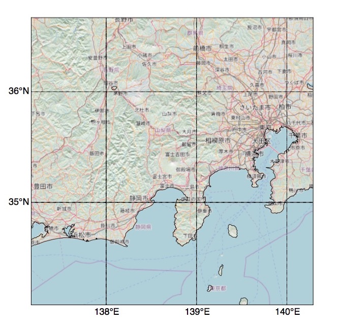
富士山周辺
北緯34.062500 東経137.170600 - 北緯36.662500 東経140.290600
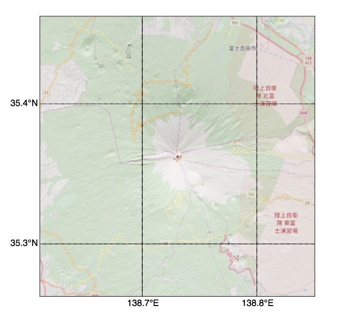
さらに拡大
北緯34.862500 東経138.130600 - 北緯35.862500 東経139.330600

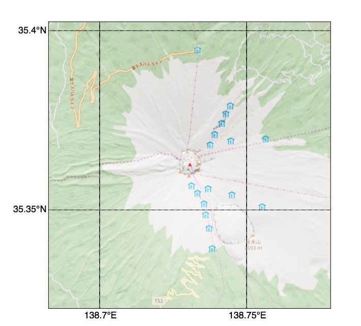
もういっちょ拡大
北緯35.262500 東経138.610600 - 北緯35.462500 東経138.850600
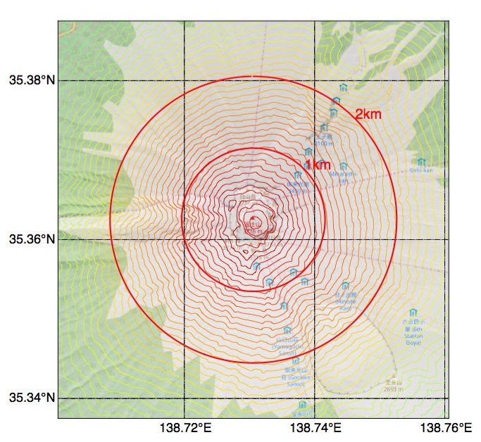
更に、しつこく拡大(笑)
北緯35.322500 東経138.682600 - 北緯35.402500 東経138.778600
宝永山や大沢崩れなどがわかりますね。
で、Pythonなので標高50m間隔で等高線を描いたり、山頂を中心に等心円を描いたりなんてことも、ほんの数行コードを追加するだけで簡単に出来ちゃったりしちゃいます。
ソースはこんな感じになります。
#!/usr/bin/env python
# -*- coding: utf-8 -*-

import requests
from StringIO import StringIO
import string
import pandas as pd
import numpy as np

import matplotlib.pyplot as plt
import matplotlib.colors as colors
from matplotlib import cm

from scipy import misc

from mpl_toolkits.basemap import Basemap
from osgeo import gdal

from math import pi
from math import tanh
from math import sin
from math import asin
from math import exp
from numpy import arctanh

from pyproj import Geod


# 1タイルのピクセル数
pix = 256

# 描画に使用する縦横の最小タイル数
Tiles = 3

g = Geod(ellps='WGS84')


# ピクセル座標を経緯度に変換する
def fromPointToLatLng(pixelLat,pixelLon, z):
    L = 85.05112878
    lon = 180 * ((pixelLon / 2.0**(z+7) ) - 1)
    lat = 180/pi * (asin(tanh(-pi/2**(z+7)*pixelLat + arctanh(sin(pi/180*L)))))
    return lat, lon


# 経緯度をピクセル座標に変換する
def fromLatLngToPoint(lat,lon, z):
    L = 85.05112878
    pointX = int( (2**(z+7)) * ((lon/180) + 1) )
    pointY = int( (2**(z+7)/pi) * (-1 * arctanh(sin(lat * pi/180)) + arctanh(sin(L * pi/180))) )
    return pointX, pointY


# 経緯度をタイル座標に変換する
def fromLatLngToTile(lat,lon, z):
    pointX, pointY = fromLatLngToPoint(lat,lon, z)
    return pointX/pix, pointY/pix


# 指定経緯度範囲が異なるタイルにまたがる最小のズームレベルとそのタイル座標を返す
def getTile(Tiles, minLat, minLon, maxLat, maxLon):

    for z in range(0,20):
        tileX1, tileY1 = fromLatLngToTile(minLat, minLon, z)
        tileX2, tileY2 = fromLatLngToTile(maxLat, maxLon, z)

        if tileX2 - tileX1 >= Tiles - 1  and tileY1 - tileY2 >= Tiles - 1: break

    return z, tileX1, tileY1, tileX2, tileY2


# 指定経緯度を中心とした指定距離範囲の経緯度の集合を返す
def createCircleAroundWithRadius(lat, lon, radiusMaters):
    latArray = []
    lonArray = []
    g = Geod(ellps='WGS84')
    for brng in range(0,360):
        a = g.fwd(lon,lat,brng,radiusMaters)

        latArray.append(a[1])
        lonArray.append(a[0])
    return lonArray,latArray


# 画像補正用シグノイド関数
def sigmoid(x):
    a = 5.0
    b = 0.4
    return 1.0 / (1.0 + exp(a * (b - x)))


# 地形データを読み込む
def load_gis(urlFormat, z, x1, y1, x2, y2):

    for x in range(x1, x2+1):
        for y in range(y2, y1+1):

            #地形データを読み込む
            url = urlFormat.format(z=z,x=x,y=y)
            print url
            response = requests.get(url)
            if response.status_code == 404:
                 Z = np.zeros((256, 256))
            else:
                 #標高値がない区画はとりあえず0mに置換する
                 maptxt = string.replace(response.text, u'e', u'0.0')
                 Z = pd.read_csv(StringIO(maptxt), header=None)
                 Z = Z.values

            # 標高タイルを縦に連結
            if y == y2:
                 gis_v = Z
            else:
                 #gis_v = cv2.vconcat([gis_v, Z])
                 gis_v = np.append(gis_v,Z,0)
                 #gis_v = np.concatenate((gis_v, Z), axis = 0) #縦

        # 標高タイルを横に連結
        if x == x1:
            gis = gis_v
        else:
            #gis = cv2.hconcat([gis, gis_v])
            #gis = np.append(gis,gis_v,1)
            gis = np.concatenate((gis,gis_v), axis = 1) #横

    return gis


# 地図画像データを読み込み各ピクセルをRGB値に変換した配列を返す
def load_imgColors(urlFormat, z, x1, y1, x2, y2):

    for x in range(x1, x2+1):
        for y in range(y2, y1+1):

            #地図画像データを読み込む
            url = urlFormat.format(z=z,x=x,y=y)
            print url
            response = requests.get(url)
            if response.status_code == 404:

                 #地図画像データが無い区画は白塗りにする
                 colors=np.ones((256, 256, 3), dtype=object)

            else:

                 #画像READ
                 img = misc.imread(StringIO(response.content))

            # 画像タイルを縦に連結
            if y == y2:
                 im_v = img
            else:
                 #im_v = cv2.vconcat([im_v, img])
                 #im_v = np.append(im_v,img,0)
                 im_v = np.concatenate((im_v, img), axis = 0) #縦

        # 画像タイルを横に連結
        if x == x1:
            im = im_v
        else:
            #im = cv2.hconcat([im, im_v])
            #im = np.append(im,im_v,1)
            im = np.concatenate((im,im_v), axis = 1) #横

    return im


def makeMap(Tiles, center_Lat, center_Lon, minLat, minLon, maxLat, maxLon):

    # 指定経緯度範囲の最適ズームとタイル座標範囲を求める
    z, x1, y1, x2, y2  = getTile(Tiles, minLat, minLon, maxLat, maxLon)


    # OpenStreetMapのタイル画像のURLフォーマット
    urlFormat = 'http://c.tile.openstreetmap.org/{z}/{x}/{y}.png'

    # OpenStreetMapのタイル画像を読み込み連結して1枚の画像として返す
    imgColors = load_imgColors(urlFormat, z, x1, y1, x2, y2)

    # 地図画像RGBデータは256で割って0..1に正規化しておく
    imgColors = imgColors/256.


    if z <= 14:
        # 標高タイルのURLフォーマット
        urlFormat = 'http://cyberjapandata.gsi.go.jp/xyz/dem/{z}/{x}/{y}.txt'

        # 標高タイルを読み込み連結して1枚の標高タイルとして返す
        Z = load_gis(urlFormat, z, x1, y1, x2, y2)


        # 勾配を求める
        (Zy,Zx) = np.gradient(Z)

        # Y軸方向の勾配を0..1に正規化
        Zgradient_norm = (Zy-Zy.min())/(Zy.max()-Zy.min())

        # Y軸方向の勾配をグレイスケール化する
        projectionIMG = cm.binary(Zgradient_norm)

        #透過情報はカット
        projectionIMG = projectionIMG[:,:,:3]

        # 地図画像と射影印影図を足して2で割りゃ画像が合成される
        imgColors = (imgColors + projectionIMG) / 2


    # 合成画像の輝度値の標準偏差を32,平均を80になんとなく変更
    imgColors = (imgColors-np.mean(imgColors))/np.std(imgColors)*32+80
    imgColors = (imgColors-imgColors.min())/(imgColors.max()-imgColors.min())

    # コントラスト補正をかける
    lut = np.empty(256)
    sigmoid0 = sigmoid(0.0)
    sigmoid1 = sigmoid(1.0)
    for i in range(256):
        x = i / 255.0
        x = (sigmoid(x) - sigmoid0) / (sigmoid1 - sigmoid0)  # コントラスト補正をかける
        lut[i] = 255.0 * x

    imgColors = np.uint8(imgColors*255)
    imgColors = lut[imgColors]
    imgColors /= 255.


    # 指定経緯度のピクセル座標を求める
    pointX1, pointY1 = fromLatLngToPoint(minLat, minLon, z)
    pointX2, pointY2 = fromLatLngToPoint(maxLat, maxLon, z)


    # 経緯度範囲に地図タイルをカット
    imgColors = imgColors[pointY2-y2*pix:pointY2-y2*pix+pointY1-pointY2, pointX1-x1*pix:pointX1-x1*pix+pointX2-pointX1, :]
    if z <= 14:
        projectionIMG = projectionIMG[pointY2-y2*pix:pointY2-y2*pix+pointY1-pointY2, pointX1-x1*pix:pointX1-x1*pix+pointX2-pointX1, :]
        Z = Z[pointY2-y2*pix:pointY2-y2*pix+pointY1-pointY2, pointX1-x1*pix:pointX1-x1*pix+pointX2-pointX1]


    # 地図を作成する
    # 3857 球面メルカトル
    # 3395 回転楕円体メルカトル
    fig = plt.figure(figsize=(12,9.8))
    map = Basemap(epsg=3857,
            lat_ts=center_Lat, resolution='h',
            llcrnrlon=minLon, llcrnrlat=minLat,
            urcrnrlon=maxLon, urcrnrlat=maxLat)


    # 背景地図画像を描画
    mx0, my0 = map(minLon, minLat)
    mx1, my1 = map(maxLon, maxLat)

    extent = (mx0, mx1, my0, my1)
    plt.imshow(imgColors, vmin = 0, vmax = 255, extent = extent)


    # 海岸線を描画
    map.drawcoastlines( linewidth=1.0, color='k' )

    # 経緯度線を描画
    map.drawparallels(np.arange(int(minLat), int(maxLat)+1, coordinateLineStep[z]), labels = [1,0,0,0], fontsize=18)
    map.drawmeridians(np.arange(int(minLon), int(maxLon)+1, coordinateLineStep[z]), labels = [0,0,0,1], fontsize=18)

    if z <= 14:
        #X,Y軸のグリッドを生成
        x = np.linspace(0, map.urcrnrx, Z.shape[1])
        y = np.linspace(0, map.urcrnry, Z.shape[0])

        X, Y = np.meshgrid(x, y)

        #標高50m間隔で等高線を描く
        #elevation = range(0,4000,50)
        #cont = map.contour(X, Y, Z, levels=elevation,linewidth=1, linestyles = 'solid', cmap='jet')
        #cont = map.contour(X, Y, Z, levels=elevation,linewidth=1, colors = '#c0d0d0', linestyles = 'solid')
        #cont = map.contour(X, Y, Z, levels=elevation,linewidth=1, colors = 'k', linestyles = 'solid')
        #cont.clabel(fmt='%1.1fm', fontsize=8)


    # 山頂を中心とした等距離円を描画
    #X, Y = createCircleAroundWithRadius(center_Lat,center_Lon,1000)
    #X, Y = map(X, Y)
    #map.plot(X,Y,marker=None,color='r',linewidth=2)
    #plt.text(X[45]+10, Y[45], '1km', fontsize=20, color='r', alpha=1.00)

    #X, Y = createCircleAroundWithRadius(center_Lat,center_Lon,2000)
    #X, Y = map(X, Y)
    #map.plot(X,Y,marker=None,color='r',linewidth=2)
    #plt.text(X[45]+10, Y[45], '2km', fontsize=20, color='r', alpha=1.00)


    plt.savefig('1.jpg', dpi=72)
    plt.show()


# ズームレベルに応じた経緯度線のステップ
coordinateLineStep = {
    5 : 5.0,
    6 : 5.0,
    7 : 2.5,
    8 : 1.0,
    9 : 0.5,
   10 : 0.25,
   11 : 0.2,
   12 : 0.1,
   13 : 0.05,
   14 : 0.02,
   15 : 0.01,
   16 : 0.005,
   17 : 0.0025,
   18 : 0.002,
   19 : 0.002
}


if __name__ == '__main__':

    # 四国
    center_Lat = 33.75
    center_Lon = 133.5


    # 富士山
    center_Lat = 35.3625
    center_Lon = 138.7306


    # 東京駅
    center_Lat = 35.681111
    center_Lon = 139.766667

    gap = 0.002
    minLat = center_Lat - gap
    minLon = center_Lon - gap * 1.2
    maxLat = center_Lat + gap
    maxLon = center_Lon + gap * 1.2

    print "北緯%f 東経%f - 北緯%f 東経%f" % (minLat, minLon, maxLat, maxLon)

    makeMap(Tiles, center_Lat, center_Lon, minLat, minLon, maxLat, maxLon)